


The process of generating a geometric mapping grid can be broken into four steps: (1) establishing a transformation (usually a polynomial), (2) testing the one-to-one property of the transformation, (3) gridding and grid reduction, and (4) the calculation of geometric errors due to the gridding process.
The process of establishing a transformation usually means a bivariate polynomial has been modeled from a set of tie point pairs (polyfit) or has been manually entered by the user. Other methods include a finite element model used in the Large Area Mosaicking System and the Projection Transformation Package as used by the remap module.
If the transformation is to be successfully applied in resample, using a geometric mapping grid, the transformation must be one-to-one. This means that each point in the output space can map to only one point in the input space and vice versa. Testing the one-to-one property is performed by the Jacobian (functional determinate) of the transformation. This test is performed in the gridgen module.
When a valid transformation has been established, it is applied to create the geometric mapping grid. The user can control the density of the mapping grid in two ways--with a default technique or by user specification.
Default Technique
The default technique is to impose a 127 x 127 grid over the output space. This maximum grid density may then be reduced using the tolval parameter. The tolval parameter contains the maximum amount (in pixels) that the linear approximated X,Y coordinates can differ from the actual grid X,Y coordinates. The grid density reduction is performed by discarding rows and columns whose grid points all have values within the tolerance value. An example using a 5 x 5 grid rather than a 127 x 127 grid follows.
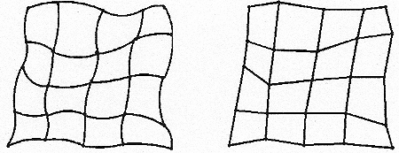
Figure G-1 illustrates the rectangular output image space mapped into the corresponding distorted input image space. Figure G-2 illustrates the linear segments that approximate the same mapping of output to input.
Figure G-1 Figure G-2
The elimination process for vertical lines (columns) and horizontal lines (rows) is done in the same way.
Elimination of vertical lines is shown in the following figures.
Figure G-3
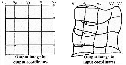
Steps:
First, test if vertical line V2 can be eliminated by drawing straight lines from the points of V1' to the points of V3' as shown. Then, according to the spacing of vertical lines V1, V2, and V3, linearly map the points on V2 ("x" marks on the straight lines).
Next, check the X and Y distances between the x-marked point and its corresponding point on V2'. The maximum of |XX'| and |YY'| is used to test against the tolerance value, where:
X, Y are coordinates of x-mark points and X', Y' are coordinates of points on V2'.
If all five maximum distances are less than or equal to the tolerance value, then drop V2 and check V3 as in the following figure.
Figure G-4
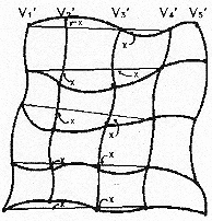
As before, connect points on V1' and V4' by straight lines and compute intermediate points. Compute distances between points on the straight line and points on V2' and V3' and check the maximum distance. If all 10 of the maximum distances are less than or equal to the tolerance value, drop V3, check V4, and so on.
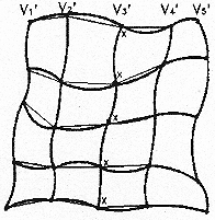
Going back to Figure G-3, if any of the five distances between the points on V2' and the points on the straight lines (connecting points on V1' and V3') is greater than the tolerance value, retain vertical line V2 and continue the process from vertical lines V2 through V5. Test V3 in the same manner as V2 was tested, and continue the process. Whenever any vertical line is to be retained, the process continues from that line.
Figure G-5
As an example, if tolval is 0.1, then the distance of the linear-approximated coordinates must be within 0.1 pixel distance of the transformation-derived coordinates. When the original transformation is linear, only vertical lines V1 and V5 are needed. On the other hand, if the transformation is highly nonlinear, no eliminations may be possible. As tolval increases, more lines can be eliminated until eventually there will be two lines (V1 and V5); however, there will be noticeable geometric distortions when resample is run and resampling generates an output image. Conversely, should tolval become smaller, more lines would be retained. If the transformation is linear, any small value for tolval gives only two vertical lines and the rest is dropped.
It should be noted that the grid expression for the transformation function is an approximation (locally linear) and reducing vertical and horizontal lines is another approximation. Also, the example given above is a simplified version of the process. Before the grid is actually reduced, resample buffering requirements are taken into consideration, often resulting in a grid which is denser than the transformation equations and the tolval parameter require it to be.
User Specification
The user has the option to specify the number of lines and samples in each grid cell. From these, the number of rows and columns in the geometric mapping grid are calculated. If the number of rows and columns exceed the maximum size of 127 x 127, the number of lines and samples in each grid cell are adjusted to fit the maximum grid size. The user is then informed of the adjustment. Using this option, it is assumed the user is aware of potential gridding errors due to grid density; grid reduction techniques are not applied.
Calculation of the errors due to the gridding process
Sixteen points (4 in X by 4 in Y) located 3/126, 43/126, 83/126, and 123/126 of the distance from one edge of the mapping grid (output space) to the other edge in both x and y dimensions are checked for errors. First, the input space coordinates of these 16 points are determined using the mapping grid. Next, the input space coordinates are recalculated using the transformation equations which were used to create the geometric mapping grid. Residual errors are then calculated between the true points (transformation derived) and the approximated points (grid derived). These residuals are written to the geometric mapping grid file and are an indication of the errors which occurred when the original transformation mapping output space to input space was gridded.
The output geometric mapping grid file contains the mapping grid point values, projection and framing information needed by resample to fill the output image's DDR (if it was available at the time of grid generation), polynomial transformation information (if a polynomial transformation was applied), as well as statistical information regarding the errors resulting from the gridding process.